Modelling An Epidemic

Sat, 23/07/2011 - 02:21 — root

Two and a half years ago, when I read the research interests of my statistics prof, I noticed that he had become interested in analyzing epidemiological models. Now, I might finally understand what he was talking about.

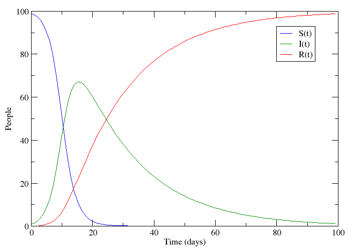
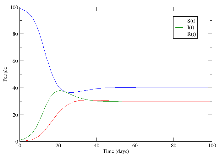
SIR model reaching the disease free equilibrium.

If we let S be the population of individuals who are susceptible to the disease, I be the population infected with it and R the population that has recovered, it is not too big a stretch to say that this plot appears to follow the progression of a non-lethal disease. Only a small number of people have the disease at the beginning, but this number grows because the disease is contagious. People who have recovered are immune to further infection meaning that the epidemic eventually dies out.

This is called an SIR-model for obvious reasons, and it is one of several compartmental models in mathematical epidemiology, developed by Kermack and McKendrick. The plot was made by numerically solving three coupled differential equations - one for each compartment. These models are of course idealized versions of the truth. Depending on what you read on the subject, you might see papers where the authors just assume that a bunch of differential equations hold. What I will try to do is motivate the assumptions that lead to this model in slightly more elegant terms.

First, we assume that all individuals in a given compartment are identical. This allows our differential equations to be ordinary differential equations. For example, the number of infected individuals only needs to be evaluated at time - $I(t)$ . Some more complicated models would use $I(t, x, a)$ telling us how many age $a$ infected individuals exist at location $x$ as a function of time.

The second assumption that is usually made is that each compartment has an exponentially distributed holding time. This makes sense because the exponential distribution is memoryless. In this case someone waiting to recover is equally likely to recover at any given time. Things like radioactive decay have taught me that exponentially distributed holding times naturally lead to rates of change that are proportional to the population size. Nevertheless, I will derive that again here because I will do something more tricky at the end of this post.

The number of individuals that recover in a given time interval is random, so the best we can do is solve for the expected number of recoveries in an interval. Whenever we model a discrete population acting randomly with a differential equation, it makes sense to use the law of large numbers. This gets us as far as:

$\begin{align*} \frac{E[\mathrm{Recovery} \; \mathrm{in} (t, t + \Delta t)]}{\Delta t} &= \frac{I}{\Delta t} P(t \leq \mathrm{Recovery} \; \mathrm{time} \leq t + \Delta t \; | \; \mathrm{Recovery} \; \mathrm{time} \geq t) \\ &= \frac{I}{\Delta t} P(\mathrm{Recovery} \; \mathrm{time} \leq \Delta t) \\ &= \frac{I}{\Delta t} F(\Delta t) \end{align*}$

where we have used memorylessness to simplify the conditional probability. We now need to know what the cumulative distribution function $F$ actually is. A quick trip to Wikipedia will tell you that:

$f(x) = \begin{cases} \gamma e^{-\gamma x} & x \geq 0 \\ 0 & x < 0 \end{cases}, \; \; \; F(x) = \begin{cases} 1 - e^{-\gamma x} & x \geq 0 \\ 0 & x < 0 \end{cases}$

We now just have to substitute this expression and Taylor expand:

$\begin{align*} \frac{\textup{d}I}{\textup{d}t} &= -\lim_{\Delta t \rightarrow 0} \frac{E[\mathrm{Recovery} \; \mathrm{in} (t, t + \Delta t)]}{\Delta t} \\ &= -\lim_{\Delta t \rightarrow 0} \frac{I}{\Delta t} \left ( 1 - e^{-\gamma \Delta t} \right ) \\ &= -\lim_{\Delta t \rightarrow 0} \frac{I}{\Delta t} \left ( 1 - \left ( 1 - \gamma \Delta t + O \left( \Delta t^2 \right ) \right ) \right ) \\ &= -\lim_{\Delta t \rightarrow 0} \left ( \gamma I + \gamma O \left ( \Delta t \right ) \right ) \\ &= -\gamma I \end{align*}$

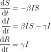
We have now expressed the decay of $I$ in terms of a recovery rate $\gamma$ . Can we do the same thing to express the decay of $S$ in terms of an infection rate $\beta$ ? Not quite. We don't want $\frac{\textup{d}S}{\textup{d}t}$ to equal $-\beta S$ because this does not account for the spread of infection. Susceptible individuals get the disease from people who already have it, so instead of using $\beta$ as our infection rate, we use $\beta I$ thus making the equations non-linear:

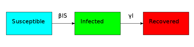
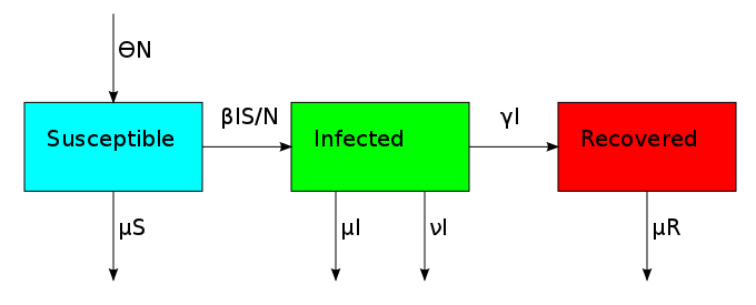
$\begin{align*} \frac{\textup{d}S}{\textup{d}t} &= -\beta I S \\ \frac{\textup{d}I}{\textup{d}t} &= \beta I S - \gamma I \\ \frac{\textup{d}R}{\textup{d}t} &= \gamma I \end{align*}$

The non-linearity makes the dynamical system hard to solve but it also allows it to reach an equilibrium point. The plot shows what is known as the disease-free equilibrium. This dynamical system is the classic starting point in formulating a whole bunch of epidemiological models. It can be summarized by a block diagram where each arrow going into a compartment contributes positively to its derivative and each arrow coming out contributes negatively.

Standard SIR block diagram.

One thing that is evident in this system is that we don't have any births or deaths. In other words, we assumed that the time scale for the disease was short. If we incorporate a death rate $\mu$ and let the birth rate be equal to it, we can explore how long lived diseases affect a population with zero net growth.

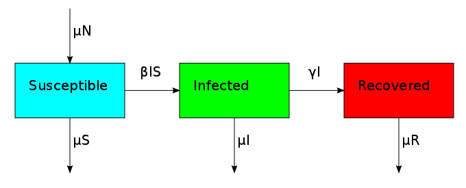
Long term SIR block diagram with zero population growth.

This changes the three compartments in an asymmetric fashion. The death rate applies equally to S, I and R, but the birth rate only replenishes S. This reflects the fact that individuals start off susceptible because they cannot have the disease when they are born. This bias creates the possibility for an additional equilibrium point called the endemic equilibrium. As shown in the next plot, the system can stabilize in a state where a finite fraction of the population permanently carries the disease.

Long term SIR model reaching the endemic equilibrium.

The bifurcation from the disease-free steady-state to the permanent epidemic occurs when a number associated with the system, $R_0$ , becomes greater than 1. The number $R_0$ , called the basic reproduction number, has a different expression for every compartmental model but it represents the number of new infections that a single infection can be expected to cause. In almost every compartmental model, the $R_0 < 1$ dynamics are much different from the $R_0 > 1$ dynamics.

There are lots of ways in which we can make the model more complicated. We can set the birth rate to $\Theta$ - something different from the death rate. When the total population changes, it is more appropriate to make the infection rate $\beta I / N$ instead of $\beta I$ (this is merely a rescaling of our $\beta$ in the previous case). We can also consider a disease where the virulence of it induces its own death rate $\nu$ .

More general SIR model.

Other common epidemiological models are SEIR (after becoming infected, there is a dormant exposed period during which a person is still unable to transmit the disease), SIS (the disease imparts no immunity and recovered individuals go back to being susceptible), SIRS (temporary immunity) and SIRC (instead of recovering, some people may become asymptomatic carriers that still infect others). In the literature, people have investigated the effects of vaccination, quarantining and biological warfare.

The last thing I want to do is choose a different distribution for the holding time. As we've described it so far, an individual moves between compartments by waiting for an exponentially distributed event to occur. I will keep it fairly simple here and have them wait for two exponentially distributed events. This means their waiting times have a gamma distribution with a shape parameter of 2 whose probability density and cumulative distribution are:

$g(x) = \begin{cases} x \gamma^2 e^{-\gamma x} & x \geq 0 \\ 0 & x < 0 \end{cases}, \; \; \; G(x) = \begin{cases} 1 - e^{-\gamma x} (\gamma x + 1) & x \geq 0 \\ 0 & x < 0 \end{cases}$

Since this distribution is not memoryless, we must evaluate the following conditional probability:

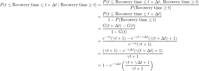$\begin{align*} P(t \leq \mathrm{Recovery} \; \mathrm{time} \leq t + \Delta t \; | \; \mathrm{Recovery} \; \mathrm{time} \geq t) &= \frac{P(t \leq \mathrm{Recovery} \; \mathrm{time} \leq t + \Delta t, \; \mathrm{Recovery} \; \mathrm{time} \geq t)}{P(\mathrm{Recovery} \; \mathrm{time} \geq t)} \\ &= \frac{P(t \leq \mathrm{Recovery} \; \mathrm{time} \leq t + \Delta t)}{1 - P(\mathrm{Recovery} \; \mathrm{time} \leq t)} \\ &= \frac{G(t + \Delta t) - G(t)}{1 - G(t)} \\ &= \frac{e^{-\gamma t}(\gamma t + 1) - e^{-\gamma t - \gamma \Delta t}(\gamma (t + \Delta t) + 1)}{e^{-\gamma t}(\gamma t + 1)} \\ &= \frac{(\gamma t + 1) - e^{-\gamma \Delta t}(\gamma (t + \Delta t) + 1)}{\gamma t + 1} \\ &= 1 - e^{-\gamma \Delta t} \left ( \frac{\gamma t + \gamma \Delta t + 1}{\gamma t + 1} \right ) \end{align*}$

With this out of the way, we are ready to find the differential equation for this process using the same method as before.

$\begin{align*} \frac{\textup{d}I}{\textup{d}t} &= -\lim_{\Delta t \rightarrow 0} \frac{E[\mathrm{Recovery} \; \mathrm{in} (t, t + \Delta t)]}{\Delta t} \\ &= -\lim_{\Delta t \rightarrow 0} \frac{I}{\Delta t} P(t \leq \mathrm{Recovery} \; \mathrm{time} \leq t + \Delta t \; | \; \mathrm{Recovery} \; \mathrm{time} \geq t) \\ &= -\lim_{\Delta t \rightarrow 0} \frac{I}{\Delta t} \left ( 1 - e^{-\gamma \Delta t} \left ( \frac{\gamma t + \gamma \Delta t + 1}{\gamma t + 1} \right ) \right ) \\ &= -\lim_{\Delta t \rightarrow 0} \frac{I}{\Delta t} \left ( 1 - \left ( 1 - \gamma \Delta t + O(\Delta t^2) \right ) \left ( \frac{\gamma t + \gamma \Delta t + 1}{\gamma t + 1} \right ) \right ) \\ &= -\lim_{\Delta t \rightarrow 0} \frac{I}{\Delta t} \left ( 1 - \frac{\gamma t + \gamma \Delta t + 1}{\gamma t + 1} + \gamma \Delta t \frac{\gamma t + \gamma \Delta t + 1}{\gamma t + 1} + O(\Delta t^2) \right ) \\ &= -\lim_{\Delta t \rightarrow 0} \frac{I}{\Delta t} \left ( \frac{\gamma^2 \Delta t (t + \Delta t)}{\gamma t + 1} \right ) \\ &= -I \frac{\gamma^2 t}{\gamma t + 1} \end{align*}$

It now seems clear to me how the differential equations must change if we wish to accommodate this new distribution:

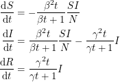$\begin{align*} \frac{\textup{d}S}{\textup{d}t} &= -\frac{\beta^2 t}{\beta t + 1} \frac{S I}{N} \\ \frac{\textup{d}I}{\textup{d}t} &= \frac{\beta^2 t}{\beta t + 1} \frac{S I}{N} - \frac{\gamma^2 t}{\gamma t + 1} I \\ \frac{\textup{d}R}{\textup{d}t} &= \frac{\gamma^2 t}{\gamma t + 1} I \end{align*}$

I have not looked hard enough to actually find these equations in print, but it would be interesting to use them and see how things change.

Tags:

fun calculations

public health

Main menu

Navigation

You are here