Main menu
You are here
Calculus On The Surface Of A Box
Lines drawn on a curved surface can be tricky. Consider one of the most basic facts about Euclidean geometry: that parallel lines never intersect. This does not hold on the surface of the Earth. If you and a friend stand one metre apart in some location on the Earth, you could both try drawing a line and heading due north. The lines would appear to be parallel during all stages of the journey but you would eventually find that they intersect at the North Pole. An observer watching from space would say that the lines don't look parallel but any measurement you could make without leaving the Earth would tell you that they are. This is because a sphere is locally flat. The fact that the lines cross can therefore be used to prove that the world is round. Similarly, measurements done in three dimensional space, might be able to prove things like that about the universe.
Now it's not just parallel lines that we have to worry about. If space were not flat, circle areas would appear to differ from  and the sum of the angles in a triangle would appear to differ from
  . There is a wonderful formalism for doing calculus with lines drawn on a curved surface and there are two contexts in which people normally learn it. One is navigation and the other is general relativity. I want to take a shot at explaining it in the context of the two ant problem. This requires us to find the shortest distance between two points on a curved surface and prove it is the shortest. So if I hadn't already solved the problem, it might seem appropriate to use the techniques that were historically used to prove that a straight line is the shortest path between two points in flat space and that a great circle is the shortest path between two points on a sphere.
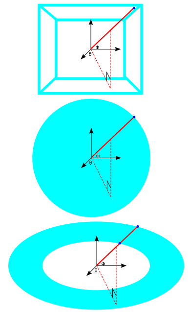
In situations like this, we should begin by choosing a co-ordinate system for our box. We will use polar co-ordinates. Those describe locations in terms of two angles  where
where  and
and  . If we wanted to describe interior points in the whole rectangular prism, the co-ordinates would be
  . This is just like how parametrize a sphere while parametrize a ball. A sphere and a box are both manifolds and they yield similar descriptions because they are homeomorphic manifolds. You may have heard that a torus is a manifold that is not homeomorphic to a sphere. One way to see why is to draw a line of constant
  and
and  . This hits two points on the torus.
Angles should label a unique point
|
A curve is a continuously indexed set of points so at time  , we can refer to our position on the path we end up taking by , we can refer to our position on the path we end up taking by  . To find the length of a curve, we can look at tiny tangents to the curve at a bunch of different times and add up all of their lengths. Therefore we want to minimize . To find the length of a curve, we can look at tiny tangents to the curve at a bunch of different times and add up all of their lengths. Therefore we want to minimize
where The standard inner product in Euclidean space just tells us that squared length is the sum of the squares of the components. Expressing this as an infinitesimal line element, it looks like:
If we are on a two-dimensional curved surface like a sphere of radius
into the Euclidean line element. What we get is:
|
![\[<br />
S = \int_{t_1}^{t_2} \left < \left ( \frac{\textup{d}\theta}{\textup{d}t}, \frac{\textup{d}\phi}{\textup{d}t} \right ), \left ( \frac{\textup{d}\theta}{\textup{d}t}, \frac{\textup{d}\phi}{\textup{d}t} \right ) \right > \textup{d}t<br />
\]](/sites/default/files/tex/589d1f79f42975689f131d8dec8f062908f718f7.png)
 and
and  are starting and ending times that we pick. Something that helps us talk about the length of a vector is an
 ![\[<br />
\textup{d}s^2 = \textup{d}x^2 + \textup{d}y^2 + \textup{d}z^2<br />
\]](/sites/default/files/tex/773bc936b9acb76c8325d0811ec324998ff2a528.png)
 anymore, we label them by
  ? No... this wouldn't make any sense. Lengths should depend on
![\[<br />
\textup{d}s^2 = r^2 \textup{d}\theta^2 + r^2 \sin^2 \theta \textup{d}\phi^2<br />
\]](/sites/default/files/tex/82aa6b18b6db854cdcb7054db8e9611879d151ea.png)
Why are we interested in the infinitesimal version of the line element? In the Euclidean case, we could have simply written  without the differentials. But for a sphere, the coefficients appearing beside the squared lengths, depend on the co-ordinate value. If we try to write down the length of a path between two points that are separated by a finite distance, the co-ordinate values would change as we moved along this path. So writing down an infinitesimal line element and integrating is what makes the most sense. Let's see if we can write down the equivalent object for a box.
In two dimensional polar co-ordinates the equation of the vertical line  is
is  . Similarly the horizontal line
  is
is  . Using this logic, an
  box can be described by:
 |
where  is the piecewise function:
![\[<br />
r(\theta) =<br />
\begin{cases}<br />
\frac{1}{\cos \theta} & -\frac{\tau}{8} \leq \theta < \frac{\tau}{8} \\<br />
\frac{1}{\sin \theta} & \frac{\tau}{8} \leq \theta < \frac{3\tau}{8} \\<br />
\frac{-1}{\cos \theta} & \frac{3\tau}{8} \leq \theta < \frac{5\tau}{8} \\<br />
\frac{-1}{\sin \theta} & \frac{5\tau}{8} \leq \theta < \frac{7\tau}{8}<br />
\end{cases}<br />
\]](/sites/default/files/tex/2738df01358dd683da22e1612c06388f64d5f7b6.png) |
We can plug this into the Euclidean line element and perform a bunch of simplifications. Since the two ant problem deals with a  box, we can also specialize to
  . After we do this, our line element for the box is still quite messy:
![\begin{align*}<br />
\textup{d}s^2 &= \left [ A \left ( r^{\prime2}(\theta) r^2(\phi) \cos^2 \theta + r^2(\theta) r^2(\phi) \sin^2 \theta - 2 r^{\prime}(\theta) r(\theta) r^2(\phi) \cos \theta \sin \theta \right ) \right \none + \\<br />
&\left \none C \left ( r^{\prime2}(\theta) \sin^2 \theta + r^2(\theta) \cos^2 \theta + 2r^{\prime}(\theta)r(\theta) \sin \theta \cos \theta \right ) \right ] \textup{d}\theta^2 + \\<br />
&A^2 \left ( r^2(\theta)r^{\prime2}(\phi) \cos^2 \theta + r^2(\theta)r^2(\phi) \cos^2 \theta \right ) \textup{d}\phi^2 + \\<br />
&2A^2 \left ( r^{\prime}(\theta) r(\theta) r^{\prime}(\phi)r(\phi) \cos^2 \theta - r^2(\theta)r^{\prime}(\phi)r(\phi) \cos \theta \sin \theta \right ) \textup{d}\theta \textup{d}\phi<br />
\end{align*}](/sites/default/files/tex/5503a63523cd15e2ee8a20cf6393efc63651fb58.png) |
This seems like a good way of getting the line element for a manifold if we know it is embedded in a higher dimensional Euclidean space. What about the inverse problem? Does every line element belong to a shape embedded in Euclidean space? The Nash embedding theorem says yes. The hyperbolic plane described by  cannot be embedded in
  . It can be embedded in
  . Whether or not four dimensions are enough is, at the time of writing, unknown.
How do we get an inner product out of this? A general inner product in finite dimensions is given by  where
where  is a symmetric, positive-definite matrix. Now notice that
  is precisely the expression:
![\[<br />
\textup{d}s^2 = [\textup{d} \theta \; \; \textup{d}\phi] \left [ \begin{tabular}{cc} g_{\theta \theta} & g_{\theta \phi} \\ g_{\theta \phi} & g_{\phi \phi} \end{tabular} \right ] \left [ \begin{tabular}{c} \textup{d}\theta \\ \textup{d}\phi \end{tabular} \right ]<br />
\]](/sites/default/files/tex/5a696c7a8c51447ea5775265e17d83f22a56c8f5.png) |
This means that from a line element, we can read off the components of a "matrix" . This bilinear map is called the metric tensor or the Riemannian metric. A manifold equipped with one of these is called a Riemannian manifold. The fact that distances on a surface are always positive forces the matrix to be positive-definite (all eigenvalues positive). As an aside, we can consider another case where one eigenvalue is negative and the rest of them are positive. This is what happens in relativity which is concerned with paths through spacetime rather than paths through space. The one negative eigenvalue corresponds to the one time direction. In this case, flat spacetime is Minkowski space rather than Euclidean space. And instead of a Riemannian manifold, we have a Lorentzian manifold. Lorentzian manifolds have given rise to a subject called causality theory.
Now that we know what our inner product is, we can go back to the integral  which gives us the length of a path joining the two ants.
![\begin{align*}<br />
S &= \int_{t_1}^{t_2} \mathcal{L} \; \textup{d}t \\<br />
\mathcal{L} &= \left [ \frac{\textup{d}\theta}{\textup{d}t} \;\; \frac{\textup{d}\phi}{\textup{d}t} \right ] G \left [ \frac{\textup{d}\theta}{\textup{d}t} \;\; \frac{\textup{d}\phi}{\textup{d}t} \right ]^{\textup{T}}<br />
\end{align*}](/sites/default/files/tex/509d79b69bd112033eb0b517c1dc501eb3a3fd96.png) |
 is the object whose integral we want to minimize. This is called a Lagrangian. Another Lagrangian that comes up a lot is the kinetic energy minus the potential energy of a mechanical system. We minimize by picking appropriate functions for . is a function that we minimize, not by plugging in a number, but by plugging in another function. Some people call this a functional. For the functional to be minimized, a necessary condition is that its functional derivative be zero. This is equivalent to solving the Euler Lagrange equations:
 |
For this particular Lagrangian, another equivalent procedure is solving the geodesic equations. The geodesic equations are usually written out in an arbitrary number of dimensions with  denoting the coordinates.
![\[<br />
\frac{\textup{d}^2x^i}{\textup{d}t^2} + \sum_{j, k} \Gamma^i_{j k} \frac{\textup{d}x^j}{\textup{d}t} \frac{\textup{d}x^k}{\textup{d}t} = 0<br />
\]](/sites/default/files/tex/47c2243005c64b83022b190773a347fc83ab6b07.png) |
The  s are called the Christoffel symbols and they can be tediously computed with the formula:
![\[<br />
\Gamma^i_{j k} = \frac{1}{2} \sum_l g^{i l} \left ( \frac{\partial g_{j l}}{\partial x^k} + \frac{\partial g_{k l}}{\partial x^j} - \frac{\partial g_{j k}}{\partial x^l}\right )<br />
\]](/sites/default/files/tex/66f5021397c1fe5efbc4d230cb181f9aa051b164.png) |
The  s with lower indices are the components of while the s with upper indices are the components of
  .
.
If we do all this for our metric on the box, we get a pair of coupled differential equations that in principle allow us to actually solve for the shortest path between two ants:
![\begin{align*}<br />
&\frac{\textup{d}^2\theta}{\textup{d}t^2} + \frac{1}{2(g_{\theta \theta} g_{\phi \phi} - g_{\theta \phi}^2)} \left [ \left ( g_{\phi \phi} \frac{\partial g_{\theta \theta}}{\partial \theta} - g_{\theta \phi} \left( 2\frac{\partial g_{\theta \phi}}{\partial \theta} - \frac{g_{\theta \theta}}{\partial \phi} \right ) \right ) \left ( \frac{\textup{d}\theta}{\textup{d}t} \right )^2 \right \none \\<br />
&+ \left \none \left ( g_{\phi \phi} \frac{\partial g_{\theta \theta}}{\partial \phi} - g_{\theta \phi} \frac{\partial g_{\phi \phi}}{\partial \theta} \right ) \frac{\textup{d}\theta}{\textup{d}t} \frac{\textup{d}\phi}{\textup{d}t} + \left ( g_{\phi \phi} \left ( 2\frac{\partial g_{\theta \phi}}{\partial \phi} - \frac{\partial g_{\phi \phi}}{\partial \theta} \right ) - g_{\theta \phi} \frac{\partial g_{\phi \phi}}{\partial \phi} \right ) \left ( \frac{\textup{d}\phi}{\textup{d}t} \right )^2\right ] = 0 \\<br />
&\frac{\textup{d}^2\phi}{\textup{d}t^2} + \frac{1}{2(g_{\theta \theta} g_{\phi \phi} - g_{\theta \phi}^2)} \left [ \left ( g_{\theta \theta} \left ( 2\frac{\partial g_{\theta \phi}}{\partial \theta} - \frac{\partial g_{\theta \theta}}{\partial \phi} \right ) - g_{\theta \phi} \frac{\partial g_{\theta \theta}}{\partial \theta} \right ) \left ( \frac{\textup{d}\theta}{\textup{d}t} \right )^2 \right \none \\<br />
&+ \left \none \left ( g_{\theta \theta} \frac{\partial g_{\phi \phi}}{\partial \theta} - g_{\theta \phi} \frac{\partial g_{\theta \theta}}{\partial \phi} \right ) \frac{\textup{d}\theta}{\textup{d}t} \frac{\textup{d}\phi}{\textup{d}t} + \left ( g_{\theta \theta} \frac{\partial g_{\phi \phi}}{\partial \phi} - g_{\theta \phi} \left ( 2\frac{g_{\theta \phi}}{\partial \phi} - \frac{\partial g_{\phi \phi}}{\partial \theta} \right ) \right ) \left ( \frac{\textup{d}\phi}{\textup{d}t} \right )^2\right ] = 0<br />
\end{align*}](/sites/default/files/tex/c994eb162cdad3f88bd90c0b954c751495a1d153.png) |
This already looks complicated and we will make it even moreso when we plug in the values that come from our complicated expression for  . Writing down a geodesic equation for a certain shape is a great way of coming up with a really complicated differential equation. A solution will exist by the Hopf-Rinow theorem but we don't have a chance in hell of being able to solve this analytically.
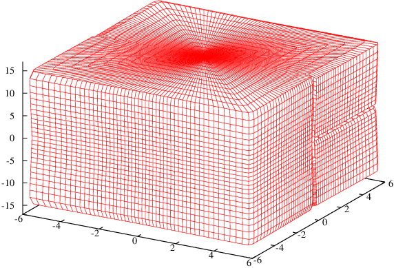
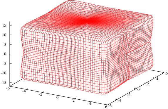
A plot I don't really trust
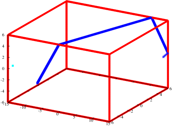
I tried to solve these equations numerically with a poor man's Euler method. In order to do this, we need initial co-ordinates. The male ant's position eleven twelfths of the way between the floor and the ceiling tells us that  . Since we are solving second order equations, we also need an initial velocity. I tried to see if the algorithm would find the length 40.7 path, so I made the initial velocity
 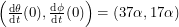 . Only the ratio of the two derivatives matters because this defines our initial direction. Geodesics obtained by using different values of
  will still chart out the same paths for the ants on the box. The ants will just cruise along them at different speeds.
Anyway, it doesn't look like this solution heads towards the female ant. I think there is some instability in the algorithm that causes the geodesic to abruptly change course when it gets to one of the edges of the box. Even if I were to get rid of this instability, a numerical simulation still cannot prove that we found the shortest path. This instability might arise because the differential equation is actually not defined on the edges. This is because our function is piecewise. I tried to approximate as a smooth function making the box lack true edges. This did not seem to help much, but it's definitely possible to invest more effort into it than I did.
In order to make  turn into
  when the angle is right, I needed to approximate a step function. Luckily, arctan does this well. Instead of going between 0 and 1, it goes between
  and
and  so we have to perform an affine transformation.
  jumps from 0 to 1 at
  if
if  is large. Now we just need a function that is periodic and positive one quarter of the time. This was hard for me to find at first because the familiar trigonometric functions are positive half of the time. The answer to this question of mathematical artistry came when I thought about Dirichlet kernels. I realized that I could just sum up cosines.
  is positive only in the region
  and we can obtain functions that are positive in the other desired regions by shifting the argument. We therefore have:
![\begin{align*}<br />
r(\theta) &= \frac{1}{\cos\theta} \left [ \arctan N \left( \cos\theta + \cos2\theta - \frac{1}{\sqrt{2}} \right ) - \arctan N \left( -\cos\theta + \cos2\theta - \frac{1}{\sqrt{2}} \right ) \right ] \\<br />
&+ \frac{1}{\sin\theta} \left [ \arctan N \left( \sin\theta - \cos2\theta - \frac{1}{\sqrt{2}} \right ) - \arctan N \left( -\sin\theta - \cos2\theta - \frac{1}{\sqrt{2}} \right )\right ]<br />
\end{align*}](/sites/default/files/tex/278320879817045ed9de58708f1797502f4e1b8d.png) |
This makes our pair of differential equations even more complicated but I think it's fun to approximate shapes like this.
We'll have to land on that small box up ahead...
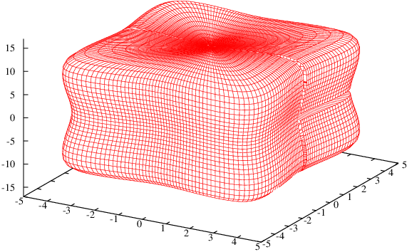
That's no box...
That's a limit of a sequence of smooth surfaces!