Main menu
You are here
Messing With Ill-Defined Physics
What's a fun thing to do when you learn a less than intuitive concept? Searching the web to find another person's opinion of it! I recently learned about Grassman numbers and my search turned up a blog post by a professor named Luboš Motl who makes some pretty debatable claims. After reading the post, I found out that he is actually quite famous. So yes, he probably knows much more than me about the subject, but I must still object to how complacent he is with using an object and not defining it.
If we know that a particle has position  at time
  ... what is the probability that we will see it at position
  at time
  ? Well in classical physics, a particle's path is fully determined so if
  lies on the path through space-time that the particle takes, this probability is 1. Otherwise it is 0. In quantum mechanics, we know this is not the case. The probability is the squared modulus of a complex probability amplitude and there are a few different ways to calculate this amplitude which may be non-trivial. Richard Feynman came up with one way that uses a phase factor:
![\[<br />
e^{iS[x(t)] / \hbar}<br />
\]](/sites/default/files/tex/d9f50f954c130dc60123a2094917b4555c589eca.png) |
His scheme requires one to integrate this phase factor over all (square integrable?) functions  satisfying
  and
and  . Functions belong to an infinite-dimensional space so this type of integral called a path integral is a little different from what we're used to. Instead of computing a double integral or a triple integral or something like that, this calculation requires us to integrate over infinitely many parameters.
In quantum field theory, the co-ordinate  should be replaced by a field
  that represents arbitrarily many particles. This agrees with Einstein's discovery that you can change how many particles you have in a system by converting some of its mass to energy:
  . If you start with the assumption that you always have one particle, you are throwing out a lot of potential physics. Now we integrate over all time-dependent fields
  such that
 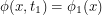 and
and  . If our particle is a boson, this is accomplished by writing as a linear combination of basis functions where each coefficient is a real number. Then we can in principle integrate all of these real numbers from
  to
to  .
.
Where am I going with this? Well if we try to describe fermions, the coefficients cannot be real numbers anymore. When we use real numbers, some of the histories we integrate over have many particles in the same state contradicting the Pauli exclusion principle. Instead, physicists have found that we get the right answer if we set the coefficients to anti-commuting numbers called Grassman numbers. At least three times, Motl has said that these numbers don't belong to any set, something that I find untrue. The two properties below that must be satisfied are anti-commutativity and associativity respectively:
 |
An immature thing I could say is that if you are even using the symbol  , you must be talking about sets - unless you're trying to rewrite all of mathematics. In fact, Grassman numbers belong to an algebra - a set where elements can be added, multiplied by scalars and multiplied by eachother. There is one subtle language convention that has to be made. Do we use the phrase "Grassman number" to refer to any element of the Grassman algebra or just the generators? Two generators
  and
and  will anti-commute but their product
  is necessarily another element of the Grassman algebra. This element commutes with a third generator
  so it is clear that not all elements of the algebra anti-commute. I will therefore only use the term "Grassman number" when referring to a generator.
What Luboš Motl meant was that the set containing Grassman numbers is not as concrete or familiar as sets like  or
or  . Is this true? Even people who stopped taking math after high school might remember that matrices are familiar objects that don't always commute. Matrices can be chosen to anti-commute and indeed if you want to represent a Grassman algebra having
  generators with matrices, you can do it as long as your matrices are
  by or larger. If we have these concrete representations, why don't physicists just use those and spare people the confusion? It's probably because we have to be able to integrate with respect to a Grassman variable
  . Since anti-commutes with itself,
  . This means that in order to integrate an analytic function
  , we need to know how to integrate
  and . Berezin's rules for doing this are:
 |
This is not what we would get if we tried to naively integrate matrices from to . Now Motl argues that people don't write limits of integration because Grassman numbers don't belong to any set. I doubt it. When a physicist omits integration limits (from a Berezin integral or a real integral) there is one reason for it: he is lazy! If you check the Wikipedia article (which I have not edited), you will see that they write an integration domain of  just like I did above. This is an exterior algebra which means that the elements inside are equivalence classes of anti-symmetric polynomials. It is up to you whether you find this concrete or not. If this exterior algebra happened to be a differentiable manifold then integration on it would be unambiguously defined for any domain - however I am pretty sure that it's not. In this sense he is right that if someone wanted to integrate over a proper subset of it would not be clear how to do it.
The operation that sends to  and to isn't really an integral. The path integral formulation for fermions makes it tempting to think of it as something analogous to the genuine integral that people use for bosons. Indeed, the following identity helps to drive that home:
![\begin{align*}<br />
\int_{\Lambda^{2n}} \theta_k \theta^{*}_l \exp \left [ -\sum_{i=1}^{n} \sum_{j=1}^{n} \theta^{*}_i A_{i, j} \theta_j \right ] \prod_{p = 1}^{n} \textup{d}\theta^{*}_p \textup{d}\theta_p &= (A^{-1})_{k, l} \int_{\Lambda^{2n}} \exp \left [ -\sum_{i=1}^{n} \sum_{j=1}^{n} \theta^{*}_i A_{i, j} \theta_j \right ] \prod_{p = 1}^{n} \textup{d}\theta^{*}_p \textup{d}\theta_p \\<br />
\int_{\mathbb{R}^{2n}} x_k x^{*}_l \exp \left [ -\sum_{i=1}^{n} \sum_{j=1}^{n} x^{*}_i A_{i, j} x_j \right ] \prod_{p = 1}^{n} \textup{d}x^{*}_p \textup{d}x_p &= (A^{-1})_{k, l} \int_{\mathbb{R}^{2n}} \exp \left [ -\sum_{i=1}^{n} \sum_{j=1}^{n} x^{*}_i A_{i, j} x_j \right ] \prod_{p = 1}^{n} \textup{d}x^{*}_p \textup{d}x_p<br />
\end{align*}](/sites/default/files/tex/1a024ca516bd9aba215935c9777ba620447035f6.png) |
Here is a new definition of the Grassman numbers that actually allows them to be integrated classically. Consider the following countable set:
![\[<br />
A = \left \{ x_p \mapsto \sin(px_p) : p \;\; \mathrm{prime} \right \}<br />
\]](/sites/default/files/tex/003135632baaa58f3152f16495bb171584f004df.png) |
Now Grassman numbers are functions on the unit circle so our integrals will at most run from to  . Now if we have a function
  from
from  to , let
 ![$ Z[f] $](/sites/default/files/tex/279ff5b86dd6fcd57dc1f6dfde5057e83a06ebd3.png) return one less than the number of
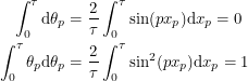
return one less than the number of  dimensional subspaces where the function vanishes. Finally, we may use the following Grassman measure and Grassman product:
![\begin{align*}<br />
\textup{d}\theta_p &\equiv \frac{2}{\tau} \sin(px_p) \textup{d}x_p \\<br />
f \star g &\equiv fg \prod_{p | Z[f]} \prod_{q | Z[g]} \textup{sgn}(p-q)<br />
\end{align*}](/sites/default/files/tex/441efaea013e7663ea479166fc4ad40b614e680d.png) |
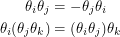
Let's see if the desired properties hold.
 |
Therefore we have anti-commutativity. Let's see if we have associativity.
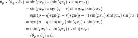 |
We have that too. And of course the integral identities work out.
 |
This allows us to integrate any analytic function with the understanding that  becomes
  . Now I can make the previously unknown claim that if I integrate
  between 0 and 0.587, the number I will get is 0.063. You might say this is all very ad-hoc. I just made up some definition involving "signs and sines" that agrees with the Berezin integral in the limiting cases and is completely unnecessary in all other cases. But the entire premise of using Grassman numbers in a path integral is also ad-hoc. Physics researchers were rightly upset that path integrals seemed like a nice object for describing bosons but not fermions. They made up definitions that would force the path integrals to work for fermions as well even though there were other perfectly good methods for doing the same calculations!
I'm also not the only person who has tried to redefine the Berezin integral. Brzezinski and Rembielinski came up with a different definition and they make it seem like my idea to integrate between and  was not far off. Their family of integrals labelled by
  behave as:
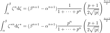 |
They point out that the Riemann integral is the case  . If we take the limit as
  , we get an integral that vanishes whenever
  just like the Berezin integral. If we want to normalize the one integral that doesn't vanish, we actually need to integrate from to
  . One paper that I couldn't manage to download proposes yet another definition that allows finite limits. I don't know what their contour integral is but I'm sure it's a well defined element of a well defined set!
Having said all this, I agree with the Bohm bashing at the end of the essay.